[SLAM Study 5주차] Fixed Map Registration과 Point-to-Plane Residual

0. 이번 주에 잡아야 하는 것

4주차에는 실제 rosbag에서 한 scan 내부의 LiDAR pose 변화가 point cloud geometry를 얼마나 바꾸는지 봤습니다.

5주차의 질문은 그 다음 단계입니다.

왜곡된 scan이 map에 붙을 때, registration residual과 inlier ratio가 어떻게 나빠지는가?

전체 연구 흐름으로 보면 이번 주 위치는 여기입니다.

quadruped gait / body motion
-> LiDAR sensor motion
-> scan distortion or deskew error
-> registration residual 증가
-> inlier ratio 감소 또는 pose update 불안정
-> mapping / odometry 성능 저하

다만 이번 5주차 실험 데이터는 로봇개 bag이 아니라 UNIST Livox 데이터입니다.

이 선택의 이유는 단순합니다. fixed-map registration residual을 보여주려면 map 구조가 선명하고 scan이 잘 보여야 합니다. Go2 야외 bag은 연구 주제와 더 직접적으로 연결되지만, 블로그 대표 그림으로는 구조가 덜 선명했습니다. 그래서 5주차는 UNIST 데이터로 evaluator를 먼저 검증하고, quadruped gait-induced motion 주장은 이후 Go2 데이터에서 다시 연결하는 흐름으로 잡습니다.

즉 5주차는 SLAM 전체를 새로 만드는 주가 아닙니다.

고정된 map에 현재 scan을 붙여 보고, scan distortion이 registration 품질 지표에 어떻게 나타나는지 측정하는 evaluator를 만드는 주입니다.

1~4주차가 여기로 이어지는 방식

5주차는 앞 주차 개념을 한 번에 다시 쓰는 지점입니다.

1주차:
  frame과 SE(3)를 알아야 scan point를 map frame으로 올릴 수 있다.

2주차:
  point time을 알아야 scan distortion과 deskew error를 말할 수 있다.

3주차:
  synthetic re-skew/deskew로 point 위치 오차가 어떻게 생기는지 분리했다.

4주차:
  실제 rosbag에서 correction magnitude와 trajectory source의 한계를 봤다.

5주차:
  그 결과가 map registration residual과 inlier ratio에 어떻게 보이는지 본다.

즉 5주차의 residual은 갑자기 나온 metric이 아닙니다.

앞에서 공부한 frame, time, deskew, trajectory estimate가 모두 맞아야 registration residual도 의미 있게 해석됩니다.

1. Registration은 무엇을 하는가

LiDAR SLAM에서 registration은 현재 scan을 이전 scan 또는 map에 맞추는 과정입니다.

가장 단순하게 말하면 다음 문제입니다.

현재 scan point들을 어떤 R, t로 움직이면
map의 표면에 가장 잘 붙는가?

여기서 $R$은 rotation, $t$는 translation입니다.

5주차에서는 full SLAM loop가 아니라 fixed map 기준의 scan-to-map registration 관점으로 봅니다.

fixed map: 이미 만들어져 있다고 가정한 reference map
current scan: 평가할 LiDAR scan
initial pose: scan을 map에 올릴 때 쓰는 초기 pose
metric: residual, inlier ratio, robust cost

이렇게 하면 map이 계속 변하는 효과를 줄이고, scan 자체의 왜곡이 registration metric에 어떻게 드러나는지 보기 쉽습니다.

Scan-to-Scan과 Scan-to-Map

registration은 크게 두 방식으로 볼 수 있습니다.

scan-to-scan:
  현재 scan을 직전 scan에 맞춘다.

scan-to-map:
  현재 scan을 누적 map 또는 fixed map에 맞춘다.

scan-to-scan은 짧은 시간 간격에서는 계산이 가볍고 drift를 바로 추정하기 좋습니다.

하지만 직전 scan도 이미 왜곡되어 있거나 pose가 틀려 있으면, 두 scan 사이의 오차가 어디서 왔는지 분리하기 어렵습니다.

scan-to-map은 더 강한 기준면을 둡니다.

현재 scan이 고정된 map 표면에 얼마나 잘 붙는가?

이번 주에는 이 질문에 집중했습니다.

그래서 fixed map은 “정답”이라기보다, 모든 scan을 같은 기준으로 비교하기 위한 reference surface입니다.

Registration은 residual 최소화 문제

registration을 수식으로 보면 결국 residual을 줄이는 문제입니다.

\[\min_{R,t} \sum_i \rho(r_i)\]

여기서 $r_i$는 각 point의 residual이고, $\rho(\cdot)$는 outlier 영향을 줄이기 위한 robust loss입니다.

이 관점에서 보면 registration 품질은 다음 세 가지가 같이 결정합니다.

1. correspondence가 맞는가?
2. residual이 작은가?
3. pose update가 안정적으로 계산되는가?

이번 5주차 evaluator는 2번과 일부 1번을 먼저 계측합니다.

아직 3번, 즉 pose update 자체를 반복해서 푸는 ICP/Gauss-Newton 단계는 넣지 않았습니다.

2. Point-to-Plane Residual

이번 주 핵심 수식은 point-to-plane residual입니다.

현재 scan의 한 point를 $\mathbf{p}_i$라고 하겠습니다.

이 point를 현재 pose $(R, t)$로 map frame에 옮기면:

\[R\mathbf{p}_i + t\]

map에서 이 point와 대응되는 local plane의 대표점을 $\mathbf{q}_i$, normal vector를 $\mathbf{n}_i$라고 하면 point-to-plane residual은 다음입니다.

\[r_i = \mathbf{n}_i^T \left( R\mathbf{p}_i + t - \mathbf{q}_i \right)\]

의미는 간단합니다.

scan point가 map의 local plane에서 normal 방향으로 얼마나 떨어져 있는가?

여기서 residual은 signed distance입니다.

하지만 metric으로 볼 때는 보통 절댓값을 봅니다.

abs residual 작음:
  scan point가 map 표면에 잘 붙음

abs residual 큼:
  scan point가 map 표면에서 많이 벗어남

point-to-plane residual은 점과 점 사이의 거리를 직접 보는 것이 아니라, map 표면의 normal 방향으로 얼마나 떠 있는지를 봅니다.

그림으로 생각하면 이런 차이입니다.

point-to-point:
  scan point와 가장 가까운 map point 사이의 3D 거리

point-to-plane:
  scan point가 map local plane에서 수직 방향으로 벗어난 거리

벽면을 예로 들면, 같은 벽 위에서 조금 옆으로 밀린 point는 point-to-point 거리로는 크게 보일 수 있습니다.

하지만 벽의 normal 방향으로는 거의 벗어나지 않았을 수 있습니다.

SLAM registration에서 더 중요한 것은 보통 “표면에서 떴는가”입니다.

그래서 벽, 바닥, 기둥처럼 표면 구조가 많은 LiDAR scene에서는 point-to-plane residual이 point-to-point residual보다 pose 보정 방향을 더 잘 줍니다.

단점도 있습니다.

한 평면만 보면 그 평면을 따라 미끄러지는 방향은 residual이 거의 변하지 않습니다.

벽 하나만 볼 때:
  벽 normal 방향 이동 -> residual이 크게 변함
  벽을 따라 이동 -> residual이 거의 안 변할 수 있음

그래서 실제 registration은 여러 방향의 벽, 바닥, 모서리, 기둥이 같이 있어야 6DoF pose가 잘 구속됩니다.

3. Correspondence와 Plane Fitting

point-to-plane residual을 계산하려면 먼저 각 scan point에 대응되는 map surface를 찾아야 합니다.

이번 evaluator의 흐름은 다음과 같습니다.

1. fixed map point cloud를 KD-tree로 만든다.
2. scan point를 initial pose로 map frame에 올린다.
3. 각 scan point 주변의 map nearest neighbor들을 찾는다.
4. neighbor point들로 local plane을 fitting한다.
5. plane normal n_i와 대표점 q_i를 얻는다.
6. point-to-plane residual r_i를 계산한다.
7. threshold로 inlier/outlier를 나눈다.

plane normal은 local map point들의 covariance를 보고 구할 수 있습니다.

작은 eigenvalue에 대응되는 eigenvector가 local plane의 normal 방향입니다.

이 부분이 중요한 이유는, residual이 단순히 두 point 사이의 거리만 보는 것이 아니기 때문입니다.

벽이나 바닥 같은 구조물에서는 point-to-plane residual이 point-to-point distance보다 registration 방향을 더 잘 설명합니다.

local plane fitting은 대략 다음 계산입니다.

주변 map point들을 $\mathbf{x}_j$라고 하면 평균은:

\[\boldsymbol{\mu} = \frac{1}{N} \sum_j \mathbf{x}_j\]

covariance는:

\[C = \frac{1}{N} \sum_j (\mathbf{x}_j - \boldsymbol{\mu}) (\mathbf{x}_j - \boldsymbol{\mu})^T\]

이 covariance의 eigenvalue를 보면 local geometry를 알 수 있습니다.

작은 eigenvalue 1개:
  점들이 한 평면 근처에 모여 있음
  해당 eigenvector가 plane normal

작은 eigenvalue 2개:
  점들이 선처럼 분포함
  normal이 불안정할 수 있음

eigenvalue 3개가 비슷함:
  local shape가 평면이라고 보기 어려움

normal 방향의 부호는 중요하지 않습니다.

$\mathbf{n}_i$ 대신 $-\mathbf{n}_i$를 써도 signed residual의 부호만 바뀌고, 절댓값 residual은 같습니다.

하지만 normal 자체가 불안정하면 residual도 흔들립니다.

따라서 sparse point, glass처럼 반사가 이상한 surface, dynamic object, map edge 근처 point에서는 correspondence와 normal을 그대로 믿으면 안 됩니다.

4. Inlier Ratio와 Residual Metric

모든 correspondence를 다 믿으면 안 됩니다.

scan point가 map 범위 밖에 있거나, 잘못된 plane에 붙거나, residual이 너무 크면 outlier로 봐야 합니다.

이번 구현에서는 크게 두 threshold를 사용했습니다.

nearest-neighbor threshold:
  fixed map에서 너무 멀리 떨어진 correspondence 제거

residual threshold:
  local plane에서 너무 멀리 떨어진 point 제거

inlier ratio는 다음입니다.

\[\mathrm{inlier\ ratio} = \frac{\mathrm{inlier\ count}} {\mathrm{correspondence\ count}}\]

5주차에서 보는 주요 지표는 다음입니다.

correspondence_count
inlier_count
inlier_ratio
residual_mean
residual_median
residual_p95
robust_cost
registration_failure

여기서 residual_p95는 특히 유용합니다.

평균은 일부 쉬운 point가 많으면 좋아 보일 수 있지만, p95는 scan에서 크게 어긋난 tail 쪽을 더 잘 보여줍니다.

이번 UNIST evaluator에서는 다음 threshold를 사용했습니다.

nn_threshold_m: 0.35
residual_threshold_m: 0.20
registration_failure threshold:
  inlier_ratio < 0.5

여기서 correspondence_count와 inlier_count는 다릅니다.

correspondence_count:
  fixed map에서 충분히 가까운 neighbor를 찾은 point 수

inlier_count:
  correspondence가 있고, residual threshold도 통과한 point 수

따라서 다음 두 상황은 서로 다릅니다.

correspondence_count가 감소:
  scan point가 map 기준으로 너무 멀어졌거나,
  map이 없는 영역으로 나갔거나,
  initial pose가 크게 틀어졌을 가능성

inlier_ratio가 감소:
  correspondence는 잡혔지만,
  local plane에서 벗어난 point가 많아졌을 가능성

robust cost는 큰 residual을 그대로 제곱해서 벌주지 않고, 일정 이상에서는 영향을 줄인 cost입니다.

이 값은 outlier에 덜 민감하지만, 반대로 p95처럼 tail 악화를 직관적으로 보여주지는 않습니다.

그래서 이번 글에서는 residual_p95와 inlier_ratio를 중심으로 해석합니다.

5. 나빠지는 방식은 하나가 아니다

이번 주에서 가장 조심해야 할 부분은 registration degradation을 한 가지 현상으로 뭉뚱그리지 않는 것입니다.

왜곡된 scan이 map에 잘 안 붙는 경우는 최소 세 가지로 나눠 볼 수 있습니다.

A. wrong plane correspondence
   - nearest neighbor distance 증가
   - correspondence 자체가 바뀜
   - inlier ratio 감소
   - residual p95 증가

B. correct plane but point location error
   - 같은 벽 또는 같은 바닥에 대응됨
   - correspondence는 유지될 수 있음
   - residual mean / median / p95 증가
   - inlier ratio는 크게 안 떨어질 수도 있음

C. geometry degeneracy
   - residual은 낮아 보일 수 있음
   - inlier ratio도 괜찮아 보일 수 있음
   - 하지만 pose update가 특정 방향으로 불안정
   - Hessian condition 또는 initial pose sensitivity가 나빠짐

그래서 registration을 볼 때는 residual 하나만 보면 부족합니다.

residual, inlier ratio, nearest-neighbor distance, pose update 안정성을 같이 봐야 합니다.

Initial Pose가 중요한 이유

registration은 보통 local optimization입니다.

처음 pose가 어느 정도 맞아 있어야 nearest neighbor도 맞고, plane normal도 맞고, residual도 의미가 있습니다.

초기 pose가 많이 틀리면 문제는 이렇게 바뀝니다.

처음 pose가 좋음:
  scan point가 실제 map surface 근처에 있음
  correspondence가 대체로 맞음
  residual이 scan distortion이나 deskew 품질을 반영함

처음 pose가 나쁨:
  scan point가 엉뚱한 wall/floor에 붙음
  correspondence가 잘못됨
  residual 증가는 scan distortion 때문인지 initial pose 때문인지 분리하기 어려움

이번 실험에서 initial_pose = identity로 고정한 이유도 여기에 있습니다.

처음부터 pose optimization까지 섞으면, residual 변화가 scan 왜곡 때문인지, optimizer가 다른 local minimum으로 간 것인지 구분하기 어려워집니다.

Gauss-Newton과 Hessian은 다음 단계

full point-to-plane ICP에서는 보통 pose update $\delta \boldsymbol{\xi}$를 반복해서 풉니다.

작은 pose 변화에 대해 residual을 선형화하면:

\[r_i(\boldsymbol{\xi} + \delta \boldsymbol{\xi}) \approx r_i(\boldsymbol{\xi}) + J_i \delta \boldsymbol{\xi}\]

전체 residual을 쌓으면 normal equation은 다음 형태가 됩니다.

\[H \delta \boldsymbol{\xi} = -g\]

여기서:

J: residual Jacobian
H = J^T J: Hessian approximation
g = J^T r: gradient

Hessian이 잘 conditioned 되어 있으면 pose update 방향이 안정적입니다.

반대로 구조가 부족하면 특정 방향이 거의 관측되지 않습니다.

예를 들어 긴 복도에서는 앞뒤 translation이나 yaw가 헷갈릴 수 있고, 큰 평면 하나만 있으면 평면을 따라 움직이는 방향이 약하게 구속됩니다.

그래서 5주차에서 말하는 geometry degeneracy는 단순히 residual이 크다는 뜻이 아닙니다.

residual은 낮아 보이지만,
pose를 어느 방향으로 고쳐야 하는지 정보가 부족한 상태

이것이 다음 주에 Hessian condition과 initial pose perturbation sweep을 보려는 이유입니다.

6. 최소 구현 구조

5주차 evaluator의 최소 코드는 다음 구조입니다.

import numpy as np
from scipy.spatial import cKDTree


def transform_points(points, R, t):
    return (R @ points.T).T + t


def point_to_plane_residuals(scan_points_map, plane_points, plane_normals):
    diffs = scan_points_map - plane_points
    return np.sum(plane_normals * diffs, axis=1)


def compute_registration_metrics(
    residuals,
    nn_distances,
    residual_threshold=0.2,
    nn_threshold=0.35,
):
    valid_corr = nn_distances < nn_threshold
    inliers = valid_corr & (np.abs(residuals) < residual_threshold)

    correspondence_count = int(np.sum(valid_corr))
    inlier_count = int(np.sum(inliers))

    if correspondence_count == 0:
        return {
            "correspondence_count": 0,
            "inlier_count": 0,
            "inlier_ratio": 0.0,
            "residual_p95": float("inf"),
            "registration_failure": True,
        }

    inlier_ratio = inlier_count / correspondence_count

    return {
        "correspondence_count": correspondence_count,
        "inlier_count": inlier_count,
        "inlier_ratio": inlier_ratio,
        "residual_p95": float(np.percentile(np.abs(residuals[valid_corr]), 95)),
        "registration_failure": inlier_ratio < 0.5,
    }

이 코드는 pose optimization을 끝까지 구현한 ICP가 아닙니다.

우선 fixed pose에서 scan이 map에 얼마나 잘 붙는지 측정하는 residual evaluator입니다.

7. UNIST Fixed-Map Registration 구현

이번 주에는 계획에서 끝내지 않고 UNIST 데이터로 최소 구현까지 만들었습니다.

구현 파일은 다음입니다.

study/fixed_map_registration.py

입력은 다음입니다.

fixed map:
/home/iamjaehka13/unist_rosbag/result/handcalib_6_24_0.mcap.ply

raw scan:
study/results/offline_deskew/unist_livox/rank_01_scan_001896/raw_time_color.ply

gyro-deskewed scan:
study/results/offline_deskew/unist_livox/rank_01_scan_001896/gyro_integrated_time_color.ply

출력은 다음 폴더에 저장했습니다.

study/results/fixed_map_registration/unist_livox_scan1896/

중요한 제한도 분명히 해야 합니다.

pose optimization: disabled
initial pose: identity
method: fixed map에 대한 point-to-plane residual evaluator

즉 이 결과는 full SLAM 결과가 아닙니다.

또한 map이 ground truth라는 뜻도 아닙니다.

다만 같은 fixed map 후보를 기준으로 raw scan, gyro-deskewed scan, synthetic distorted scan의 registration metric을 비교할 수 있습니다.

8. 대표 3D 그림이 의미하는 것

5주차 대표 그림은 VTK로 다시 렌더링한 vtk_low_oblique_residual_triptych.png입니다.

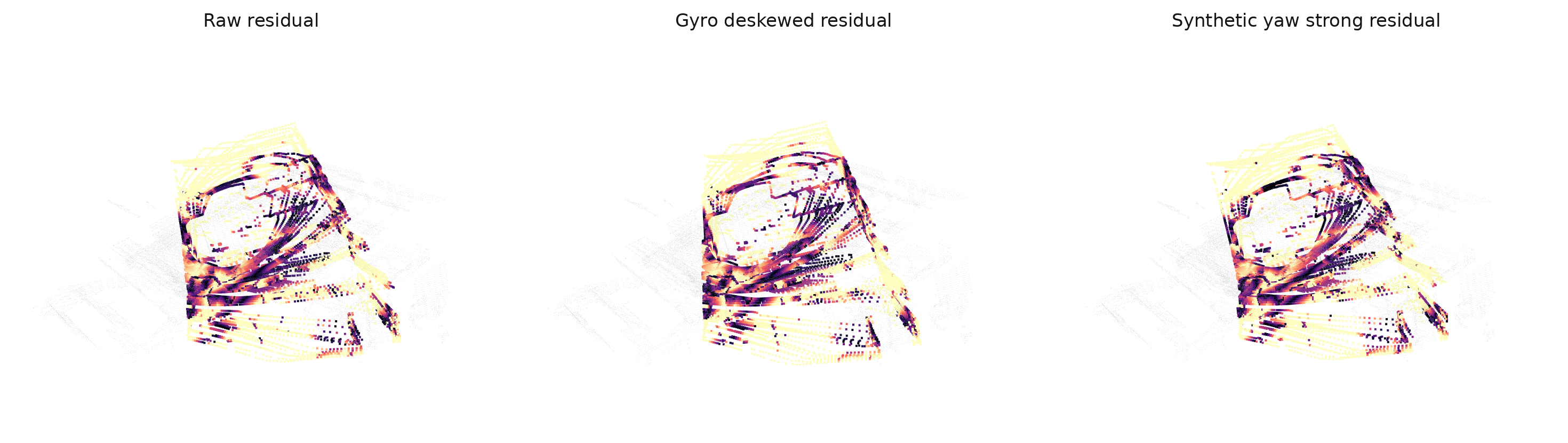
이 그림은 세 개의 scan을 fixed map 위에 올려 놓고 비교한 것입니다.

left:
  raw scan

middle:
  gyro-integrated deskewed scan

right:
  synthetic yaw strong 6 deg distortion scan

회색 점들은 fixed map입니다.

색이 입혀진 점들은 평가 대상 scan point입니다.

색은 point-to-plane residual의 절댓값을 의미합니다.

어두운 색:
  fixed map의 local plane에 비교적 잘 붙은 point

밝은 노란색:
  fixed map의 local plane에서 많이 벗어난 point

따라서 이 그림은 “deskew가 예쁘게 됐다”를 직접 증명하는 그림이 아닙니다.

정확히는 다음을 보여주는 그림입니다.

같은 fixed map 기준으로 볼 때, 각 scan point가 local plane에서 얼마나 떨어져 있는가?

그래서 5주차 글에서는 이 그림을 registration residual 분포를 보는 진단 그림으로 해석해야 합니다.

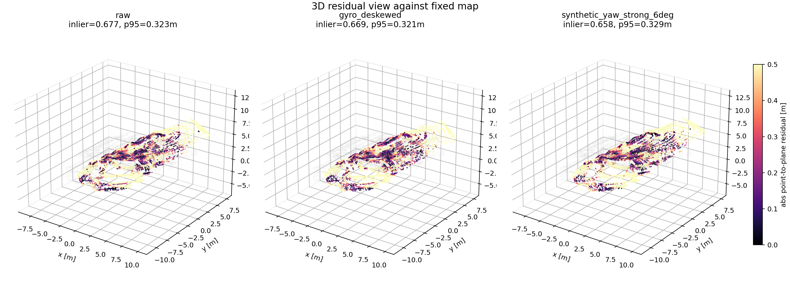
처음 matplotlib 3D 그림만 보면 데이터가 2D처럼 보일 수 있습니다. 하지만 데이터 자체는 2D가 아닙니다.

fixed map z span: 8.252 m
raw scan z span: 8.837 m
gyro-deskewed scan z span: 8.814 m

2D처럼 보였던 이유는 point cloud가 빈 공간을 채우는 volume data가 아니라, 벽, 바닥, 구조물 표면을 샘플링한 surface data이기 때문입니다. 즉 LiDAR point cloud는 3D 좌표를 갖지만, 시각적으로는 얇은 표면들의 집합처럼 보이는 것이 자연스럽습니다.

보조로 축과 colorbar가 있는 matplotlib 3D 그림도 남겨 둡니다. 수치 비교를 읽기에는 이 그림이 더 직접적입니다.

9. 주요 수치

이번 evaluator에서 나온 핵심 수치는 다음입니다.

method	correspondence	inlier ratio	residual median m	residual p95 m	robust cost
raw	7552	0.676642	0.139484	0.323333	159.419073
gyro_deskewed	7512	0.668530	0.144108	0.320903	163.167669
synthetic_yaw_weak_1deg	7553	0.672580	0.139471	0.324349	159.586067
synthetic_yaw_medium_3deg	7513	0.670571	0.140490	0.323749	159.274829
synthetic_yaw_strong_6deg	7458	0.658219	0.146841	0.329254	162.083715

시각적으로 보면 다음과 같습니다.

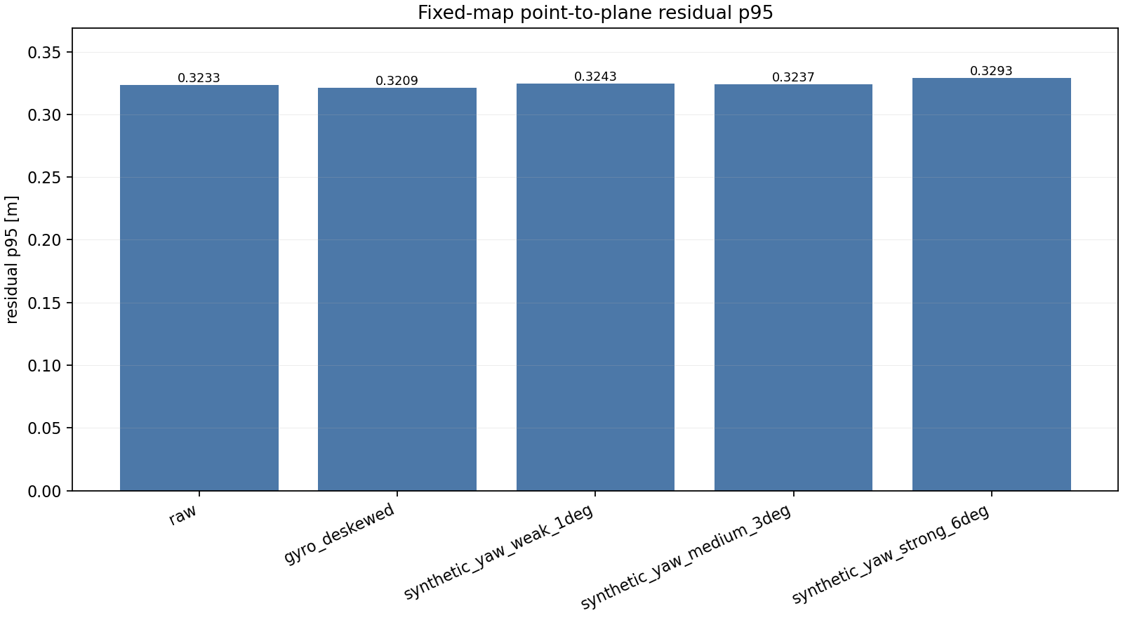
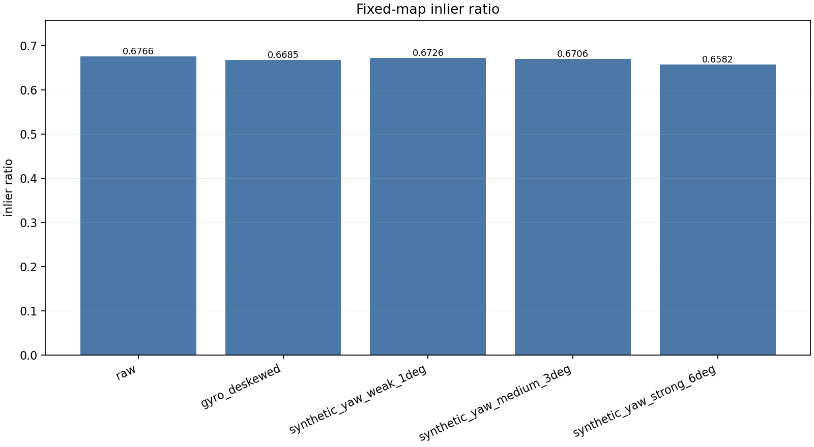
가장 중요한 비교는 raw와 synthetic strong입니다.

raw:
  residual p95 = 0.323333 m
  inlier ratio = 0.676642

synthetic_yaw_strong_6deg:
  residual p95 = 0.329254 m
  inlier ratio = 0.658219

strong synthetic yaw distortion은 raw보다 residual p95가 커지고, inlier ratio가 낮아졌습니다.

즉 controlled distortion이 fixed-map registration metric을 악화시키는 방향은 확인됐습니다.

이 표에서 읽어야 하는 포인트는 세 가지입니다.

첫째, raw와 gyro-deskewed의 차이는 매우 작습니다.

raw residual p95:
  0.323333 m

gyro_deskewed residual p95:
  0.320903 m

rotation-only gyro deskew가 p95 residual을 약간 줄였지만, inlier ratio는 오히려 raw보다 낮습니다.

이것은 이상한 결과라기보다, 현재 evaluator의 한계를 보여주는 결과입니다.

1. translation deskew는 들어가지 않음
2. fixed map이 ground truth는 아님
3. initial pose를 identity로 고정함
4. residual은 local plane fitting과 correspondence 선택에 민감함

즉 gyro-deskewed가 모든 metric에서 이겨야 한다고 기대하면 안 됩니다.

둘째, synthetic strong은 raw보다 더 나쁜 방향으로 움직였습니다.

raw inlier ratio:
  0.676642

synthetic strong inlier ratio:
  0.658219

같은 fixed map, 같은 evaluator에서 강한 artificial yaw distortion을 넣었을 때 inlier ratio가 떨어졌습니다.

이 부분이 5주차의 핵심 관찰입니다.

셋째, residual p95와 inlier ratio는 서로 보완적입니다.

residual p95는 살아남은 correspondence들 중 tail이 얼마나 나쁜지 보여줍니다.

inlier ratio는 threshold를 통과한 point가 얼마나 남았는지 보여줍니다.

따라서 좋은 registration은 보통 다음 형태를 기대합니다.

residual p95 낮음
inlier ratio 높음
correspondence_count 충분함
robust cost 낮음
pose update 안정적

이번 구현은 이 중 pose update 안정성까지는 아직 보지 않았습니다.

10. 조심해야 하는 해석

이번 결과에서 가장 조심할 점은 다음입니다.

residual p95 = SLAM error가 아님
inlier ratio = 최종 localization 성능이 아님
UNIST fixed map = ground truth map이 아님
gyro_deskewed 결과 = 항상 raw보다 좋아야 하는 reference가 아님

특히 gyro-deskewed scan은 raw보다 p95 residual은 약간 작지만, inlier ratio와 robust cost는 더 좋아졌다고 말하기 어렵습니다.

따라서 이번 결과를 이렇게 쓰면 안 됩니다.

gyro deskew가 registration 성능을 검증했다
deskew로 SLAM 정확도가 개선됐다
fixed map residual이 ground-truth error다

안전한 표현은 다음입니다.

UNIST fixed map 후보를 기준으로 scan-to-map residual evaluator를 만들었고,
strong synthetic yaw distortion에서 raw보다 p95 residual 증가와 inlier ratio 감소가 관찰됐다.

또 하나 중요한 점은 synthetic distortion sweep이 완전히 단조적이지 않았다는 것입니다.

weak, medium, strong 순서로 residual p95와 robust cost가 항상 증가하지는 않았습니다.

그래서 “distortion이 강해질수록 모든 metric이 단조적으로 나빠졌다”라고 쓰면 안 됩니다.

현재 말할 수 있는 결론은 더 제한적입니다.

strong synthetic distortion은 raw 대비 fixed-map residual/inlier metric을 악화시키는 사례를 만들었다.

11. 5주차 결과물

이번 주 결과물은 다음입니다.

study/fixed_map_registration.py

study/results/fixed_map_registration/unist_livox_scan1896/
  registration_metrics.csv
  summary.md
  vtk_low_oblique_residual_triptych.png
  spatial_residual_3d.png
  spatial_inlier_3d.png
  residual_p95_bar.png
  inlier_ratio_bar.png
  residual_histogram.png
  *_residual_color.ply
  *_inlier_color.ply

이번 구현의 역할은 명확합니다.

input:
  fixed map + scan

output:
  point-to-plane residual
  inlier ratio
  robust cost
  residual-colored visualization

아직 하지 않은 것은 다음입니다.

Gauss-Newton pose update
multi-iteration ICP
external odometry validation
true ground-truth map comparison
SLAM trajectory drift comparison

12. 다음 단계

다음 주에 더 강한 결과로 가려면 fixed-pose residual evaluator에서 pose optimization으로 넘어가야 합니다.

우선순위는 다음입니다.

1. point-to-plane Jacobian 구현
2. Gauss-Newton pose update 추가
3. initial pose perturbation sweep
4. Hessian condition으로 geometry degeneracy 확인
5. raw / deskewed / synthetic distortion의 convergence 비교
6. 가능하면 외부 odometry 또는 SLAM 결과와 비교

이렇게 해야 registration metric 변화가 단순 residual 진단을 넘어서 실제 pose estimation 안정성까지 이어지는지 볼 수 있습니다.

13. 이번 주 요약

5주차는 다음 한 문장으로 정리됩니다.

deskew된 scan 또는 왜곡된 scan이 fixed map의 local plane에 얼마나 잘 붙는지를 point-to-plane residual과 inlier ratio로 측정하는 주였다.

핵심은 residual이 커졌다는 사실만 보는 게 아닙니다.

왜 커졌는지, correspondence가 깨진 것인지, 같은 plane 위에서 point 위치만 흔들린 것인지, 아니면 geometry가 애초에 pose update를 잘 구속하지 못하는 것인지 구분하는 것이 중요합니다.

이번 UNIST 결과는 그 분석으로 가기 위한 첫 evaluator입니다.

아직 연구 claim으로 세게 쓰면 안 되지만, 4주차 deskew 시각화에서 5주차 registration degradation 분석으로 넘어가는 연결고리로는 충분합니다.